Execution Plans, Caching, partitioning and Gloming.
Lazy Evaluation
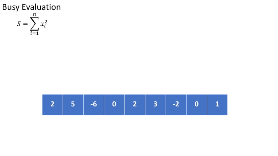
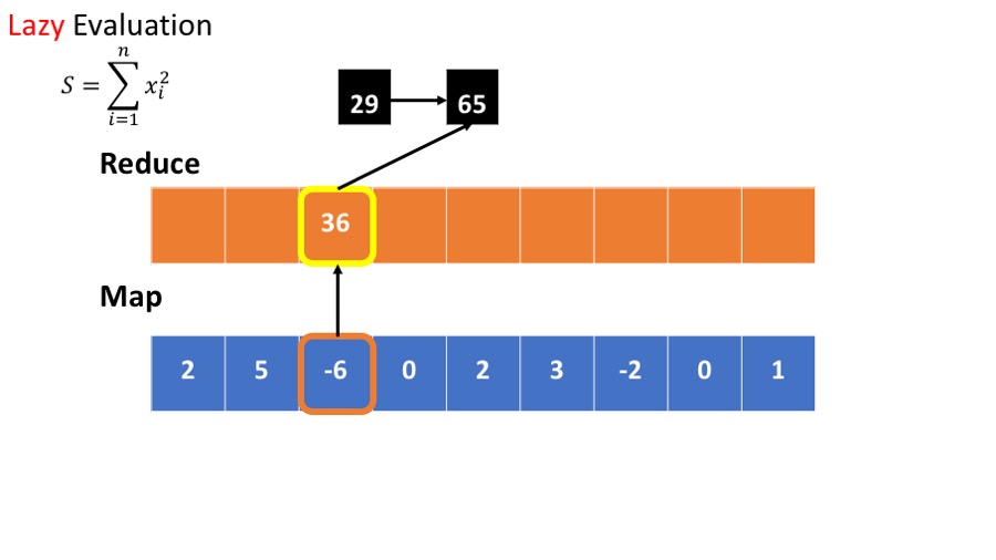
- we want to calculate the sum of he squares : $\sum_{i=1}^n x_i^2 $
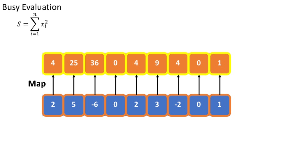
The standard (or busy) way to do this is
- Calculate the square of each element.
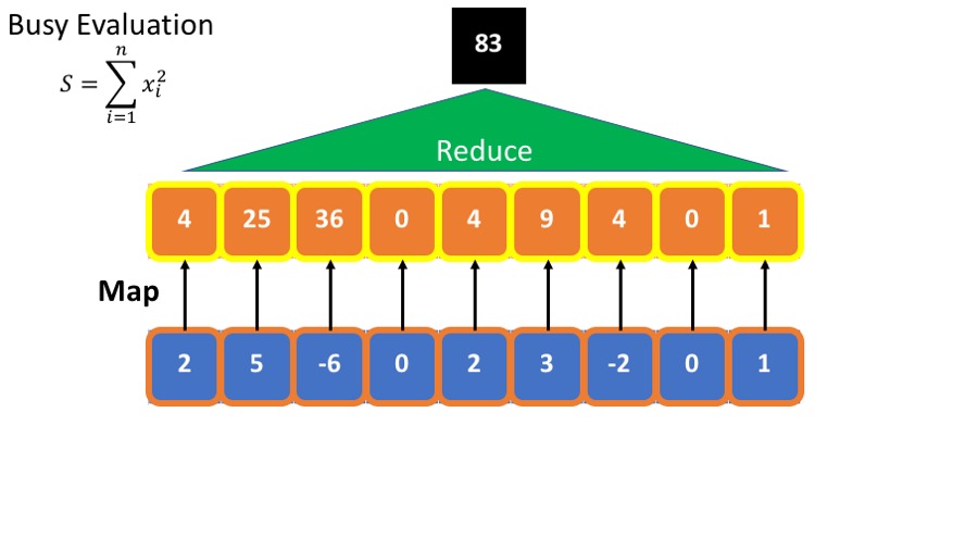
- Sum the squares.
This requires storing all intermediate results.
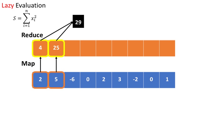
An alternative is lazy evaluation:
- postpone computing the square until result is needed.
- No need to store intermediate results.
- Scan through the data once, rather than twice.
Experimenting with Lazy Evaluation
import findspark
findspark.init()
from pyspark import SparkContext
sc = SparkContext(master="local[3]")  #note that we set the number of workers to 3
Demonstration of lazy evaluation
We create an RDD with one million elements so that the effect of lazy evaluation and caching is significant.
%%time
RDD=sc.parallelize(range(1000000))
It takes about 01.-0.5 sec. to create the RDD.
Define a computation
The role of the function taketime is to consume CPU cycles.
from math import cos
def taketime(i):
    [cos(j) for j in range(10)]
    return cos(i)
%%time
taketime(5)
define the map operation.
- Note that this cell takes very little time.
- Because lazy evaluation delays actual computation until needed.
%%time
Interm=RDD.map(lambda x: taketime(x))
- Why did the previous cell took less than 50 micro-seconds (Wall Time)?
- Bcause no computation was done
- The cell defined an execution plan, but did not execute it yet.
Execution Plans
At this point the variable Interm does not point to an actual data structure. Instead, it points to an execution plan expressed as a dependence graph. The dependence graph defines the dependence of the RDD on each other.
The dependence graph associated with an RDD can be printed out using the method toDebugString().
The first line corresponds to Interm and the second line corresponds to RDD which is the input to Interm
print Interm.toDebugString()
At this point only the two left blocks of the plan have been declared.
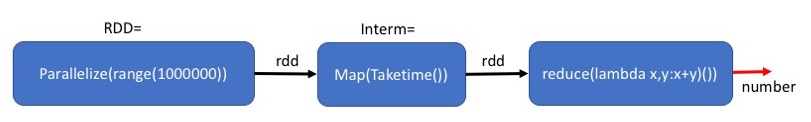
Actual execution
The reduce command needs to output an actual output, spark therefor has to actually execute the map and the reduce. Some real computation needs to be done, which takes about 1 - 3 seconds (Wall time) depending on the machine used and on it's load.
%%time
print 'out=',Interm.reduce(lambda x,y:x+y)
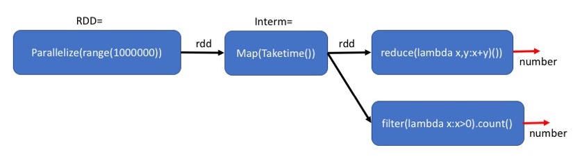
Executing a different calculation based on the same plan.
The plan defined by Interm can be executed many times. Below we give an example.
Note: the run-time is similar to that of the previous command because the intermediate results that are due to Interm have not been saved in memory.
%%time
print 'out=',Interm.filter(lambda x:x>0).count()
The middle block: Map(Taketime) is executed twice. Once for each final step.
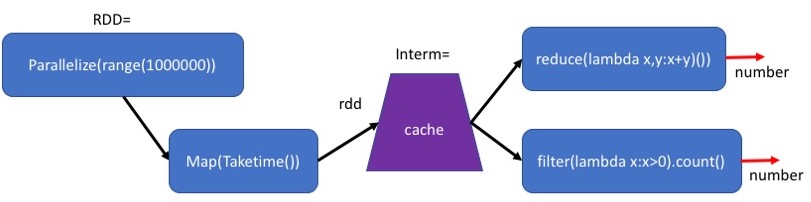
Caching intermediate results
The computation above is wasteful because each time we recompute the map operation.
We sometimes want to keep the intermediate results in memory so that we can reuse them without recalculating them. This will reduce the running time, at the cost of requiring more memory.
The method cache() indicates that the RDD generates in this plan should be stored in memory. Note that this is still only a plan. The actual calculation will be done only when the final result is seeked.
%%time
Interm=RDD.map(lambda x: taketime(x)).cache()
By adding the Cache after Map(Taketime), we save the results of the map for the second computation.
Plan to cache
The definition of Interm is almost the same as before. However, the plan corresponding to Interm is more elaborate and contains information about how the intermediate results will be cached and replicated.
Note that PythonRDD[4] is now [Memory Serialized 1x Replicated]
print Interm.toDebugString()
Creating the cache
The following command executes the first map-reduce command and caches the result of the map command in memory.
%%time
print 'out=',Interm.reduce(lambda x,y:x+y)
Using the cache
This time Interm is cached. Therefor the second use of Interm is much faster than when we did not use cache: 0.25 second instead of 1.9 second. (your milage may vary depending on the computer you are running this on).
%%time
print 'out=',Interm.filter(lambda x:x>0).count()
Partitioning and Gloming
When an RDD is created, you can specify how many partitions it should have. The default is the number of workers defined when you set up SparkContext
A=sc.parallelize(range(1000000))
print A.getNumPartitions()
We can repartition A into a different number of partitions.
The method .partitionBy(k) expects to get a (key,value) RDD where the keys are integers.
it will put in partition i all of the element for which key%k == i
B= A.map(lambda x: (2*x,x)) \
    .partitionBy(10)
print B.getNumPartitions()
glom() transforms each partition into a tuple (immutabe list) of elements.
As they are tuples, the workers can refer to elements of the partition by index. (but you cannot assign values to the elements, the RDD is still immutable)
def getPartitionInfo(G):
    d=0
    if len(G)>1:
        for i in range(len(G)-1):
            d+=abs(G[i+1][1]-G[i][1]) # access the glomed RDD that is now a  list
        return (G[0][0],len(G),d)
    else:
        return(None)

output=B.glom().map(lambda B: getPartitionInfo(B)).collect()
print output
Note that the odd numbered partitions are empty. Why is that?
Repartitioning for Load Balancing
Suppose we start with 10 partitions, all with exactly the same number of elements
A=sc.parallelize(range(1000000))\
    .map(lambda x:(x,x)).partitionBy(10)
print A.glom().map(len).collect()
As we process the RDD, we find that most of the useful elements are in a single partition.
We simulate this using a filter() command that filters out all of the elements from all but one of the partitions.
#select 10% of the entries
B=A.filter(lambda (k,v): k%10==0)
# get no. of partitions
print B.glom().map(len).collect()
Left unchecked, the result is that all of the computation is done by a single worker.
To fix the situation we need to repartition the RDD.
One way to do that is to repartition using a new key.
C=B.map(lambda (k,x):(x/10,x)).partitionBy(10)
print C.glom().map(len).collect()
Another approach is to use random partitioning.
- An advantage of random partitioning is that it does not require defining a key.
- A disadvantage of random partitioning is that the size of the partitions is only approximately equal.
D=B.repartition(10)
print D.glom().map(len).collect()